
1. Introduction
Lynx Seismap is an ESRI ArcMap extension for viewing 2D and 3D seismic datasets, wireline logs and raster cross-sections. Lynx Seismap currently supports ArcGIS Desktop versions 10.6, 10.5, 10.4, 10.3, 10.2, 10.1 and 10.0
2D seismic profiles, 3D seismic inlines and crosslines, wireline logs and raster cross-sections are displayed in separate independent windows. Current visible shotpoint/CDP ranges or cross-section extents are tracked on the map. Multiple profiles, well logs and cross-sections can be viewed simultaneously, surfaces can be overlaid on the seismic profile as horizons and faults, and well formation tops displayed with the wireline curves. Each viewer allow extensive control over the display scales and zooming, many different display options, printing to full-scale windows-compatible plotters, quick setting of shotpoint basemap annotation options, and import and export of gridded surfaces and horizons.
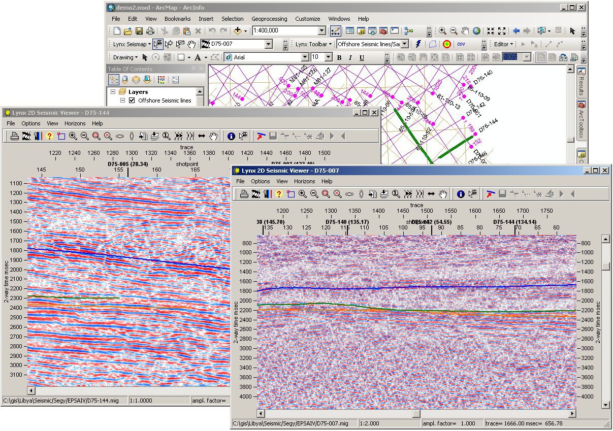
The screenshot above shows a 2D seismic basemap in the ArcMap main window, and two seismic viewer windows displaying 2D profiles in colour display mode, with horizon overlays.
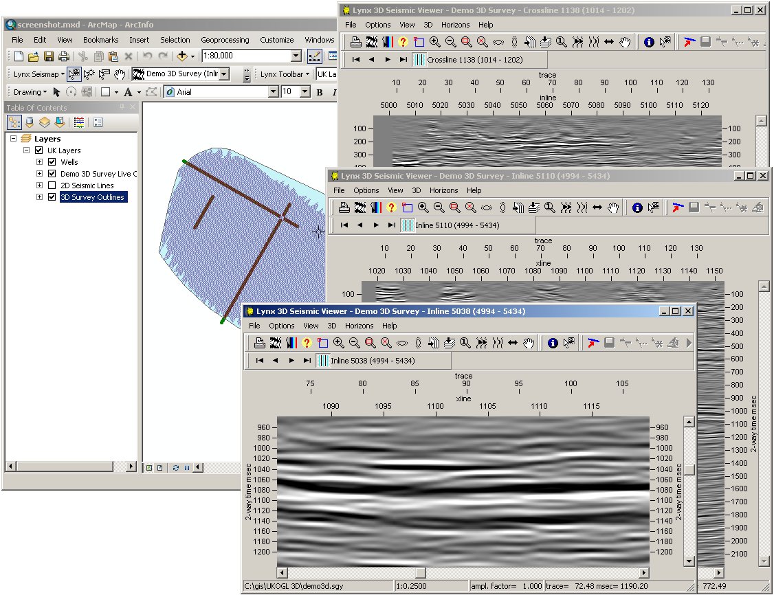
The screenshot above shows a 3D seismic survey polygon (overlaid with live traces) in the main ArcMap window, with seismic viewer windows showing two inlines and one crossline in greyscale display mode
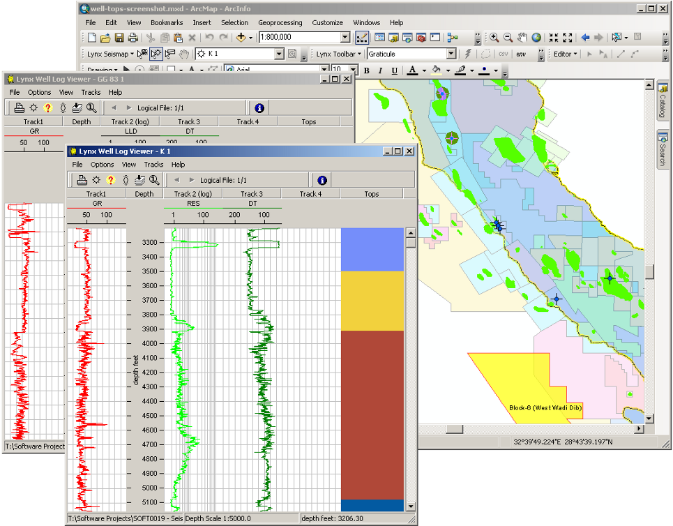
The screenshot above shows the wireline curves from two wells with a well tops column.
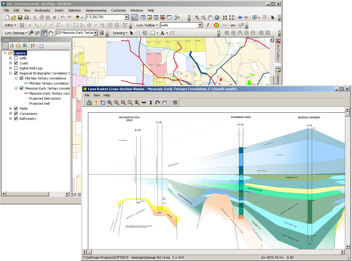
The screenshot above shows the cross-section viewer with highlighted section in Arcmap's main window
The prerequisites for Seismap are similar to those required for standard ArcMap field-based hyperlinks.
For 2D seismic data, Seismap requires a polyline-M feature class or route event containing the seismic locations. Each 2D seismic profile is a separate feature, with shotpoints stored as the measure values. The attribute table should contain a field which contains the file-path targets for the seismic data. The seismic files can be either SEG-Y (Revision-1 or Standard) or Lynx TR-files.
For 3D seismic data, Seismap requires a feature class containing a polygon outlines of each 3D survey, with inline and crossline numbers stored for each vertex as ID & M (or Z & M) values. As with 2D data, the attribute table should contain a field which contains the file-path target. Each 3D survey is stored as a single feature. The seismic data should be stored in a single SEG-Y file per survey, sequential inlines stored end-to-end, with ascending crossline numbers for each inline. It is not necessary to pad all inlines to the same number of traces. Inline and crossline numbers should be stored in the trace headers of the seismic data.
Gridded horizon surfaces can be stored as either raster grids or TINs. If you wish to use TIN surfaces to display horizon overlays on your seismic profiles, you must have the ESRI 3D Analyst extension installed and licensed (however, raster grid surfaces do not require the 3D Analyst extension).
For wireline data, Seismap requires a point feature class of the well surface locations. Each well is a separate feature. The attribute table should contain a field which contains the file-path targets for the wireline data, which can be in LAS or LIS formats.
For cross-sections, Seismap requires a polyline feature class of the surface-locations of the cross-sections, with each cross-section as a separate feature. The attribute table should contain a field which contains the file-path targets of each cross-section, which can be in one of the following formats: TIFF(RGB), JPEG, PNG, BMP, PDF.
2. Installation, Licensing and Activation
2.1 Installation
Lynx Seismap is a COM DLL extension for ESRI ArcMap, and requires ArcMap version 10.6, 10.5, 10.4, 10.3, 10.2, 10.1 or 10.0 to be installed and licensed for use on your PC. Seismap uses the same components for viewing seismic data as the Lynx Seismic Viewer SEISVIEW, and the default installation folder will be your existing LYNXSYS folder. For standalone installations, the setup wizard will register Seismap as a COM server and as an ArcMap extension. This COM registration may require administrative privileges on your PC.
Lynx Seismap can also be manually installed on client PCs - copy the installed contents of the LYNXSYS folder, and register the main DLL using the following commands:
Register seismap10.dll using the ESRI utility ESRIRegAsm.exe (usually installed into %CommonProgramFiles%\ArcGIS\bin):
ESRIREGASM path\to\SEISMAP10.DLL /p:Desktop /s
Seismap may also be registered on a client PC by using the Lynx FILEREG utility from the Lynx Launcher.
The horizon polyline feature renderer uses the Microsoft GDI+ graphics engine. The setup wizard will install it if required.
2.2 Licensing
When first installed, Seismap will be licensed for a trial period. After this trial period expires, Seismap will require a Lynx program licence in order to run. See Lynx Software Licensing for details of the different licensing mechanisms available.
Seismap modules are licenced separately:
- Viewers for 2D seismic lines, 3D seismic inlines and crosslines, wireline logs and raster cross-sections
- Import and export of SEG-P1/UKOOA for 2D seismic lines, 3D seismic survey polygon from trace headers, ZMap, horizons and faults. Import of wireline logs and raster/PDF cross-sections.
The licence checker is activated when a seismic viewer window or import/export tool is opened, and de-activated when all Seismap windows are closed.
You can request a licence activation on-line at Lynx's website (http://www.lynxinfo.co.uk/download-licence.html) to enable Seismap after the trial period has expired.
2.3 Activation
The Seismap extension can be activated and deactivated in ArcMap
in the standard way by using Extensions dialog. This is accessed in ArcMap 10
via the Customize-Extensions menu. You should ensure that the Lynx Seismap
extension is enabled before an MXD containing a stored Seismap configuration
is opened, otherwise the stored configuration will not be read from the MXD, and
default values will be used.
The Seismap toolbar (see below) is
enabled and disabled along with the extension. If the toolbar is not visible
when you open ArcMap, use the Customize-Toolbars menu in Arcmap to display
the Toolbars list, and check the entry for the Lynx Seismap Toolbar.
3. Lynx Seismap Toolbar
Seismap installs a toolbar into ArcMap (see Activation, above). This contains the tools for activating the Seismap viewers for 2D and 3D seismic data, wireline logs and raster cross sections
-
Select Seismic Profile
 tool
tool
When you have valid layers specified as your 2D and/or 3D seismic basemap layers, this tool can be activated. The map cursor will change to indicate that you can select a seismic 2D profile or 3D inline/crossline by clicking it on the map. For details see below. -
Select Well
 tool
tool
When you have valid layers specified as your well locations, this tool can be activated. The map cursor will change to indicate that you can select a well by clicking it on the map. For details see below. -
Select Cross-Section
 tool
tool
When you have valid layers specified as your raster cross-section layers, this tool can be activated. The map cursor will change to indicate that you can select a cross-section profile by clicking it on the map. For details see below. -
Pan Viewer
 tool
tool
When at least one seismic viewer window is displayed, this tool can be activated. You can pan a viewer window by clicking its current highlighted range on the map and dragging it to the range you wish to display. -
Current Objects combo box.
This combo-box displays all the current open 2D and 3D seismic profiles, wells and raster cross-sections. To bring a viewer window to the front, select it from the drop-down list. -
Zoom to Current Object

Zoom the map display to the active seismic profile/well/cross-section (the one selected in the Current Object combo box). - Lynx Seismap menu
- Seismic Display Options

Set display and scale parameters globally for all seismic 2D and 3D viewer windows.
See Seismic Display Parameters (below) for details. - Wireline Display Options

Set display and scale parameters globally for all wireline viewer windows.
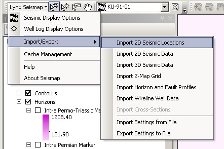
See Wireline Display Parameters (below) for details. - Import/Export
- Import 2D Seismic Locations
Convert a UKOOA/SEG-P1 file or CSV file containing shotpoint/CDP coordinates into a shape file. See Import 2D Seismic Locations (below) for details. - Import 2D Seismic Data
Select seismic data (SEG-Y) files to display with Seismap. See 2D Seismic Data Import (below) for details. - Import 3D Seismic Data
Select 3D seismic data files to generate survey outline polygons and display inlines and crosslines with Seismap. See 3D Seismic Data Import (below) for details. - Import Z-Map Grid
Read a Z-Map ASCII grid file and create a file geodatabase grid or ESRI raster grid. This allows you to import gridded horizon and fault data from seismic interpretation systems. See Z-Map Grid Import (below) for details. - Import Horizon and Fault Profiles
Read ASCII files containing interpreted horizon or fault data. The ASCII files can contain an interpreted horizon/fault for a single seismic profile, or for a number of different seismic profiles. See Horizon/Fault Import and Export for details. The imported horizons will be displayed on the map using Seismap's custom polyline-Z feature renderer using a colour ramp, and will also be displayed in seismic viewer windows. - Import Wireline Well Data
Select LAS/LIS wireline log files to display with Seismap. See Wireline Log Import (below) for details. - Import Cross-Sections
Select raster or PDF images to display with Seismap. See Cross-Section Import (below) for details. - Import Settings from File
Load a Seismap parameter file previously exported from ArcMap. Seismap parameter files are stored with extension .asv. Browse for the file to open from the standard Open File dialogue. The Seismic Display Parameters and Wireline Display Parameters will be imported from the specified file,.and saved into the current MXD file. - Export Settings to File
Save the current Seismap parameter set to an external file. Set the filename in the standard Save File dialogue. Seismap parameter files are stored with extension .asv. Use this option to share seismic and wireline display/scale between ArcMap projects.
- Import 2D Seismic Locations
- Cache Management
Seismap stores 2D profile, horizon and well intersection information, plus 3D-seismic inline and crossline indexes, and 3D-seismic survey calibrations after their initial calculation, for quick retrieval. The options in this dialog can be used to clear the cached data, which may be required after editing layers, or if the display map projection is changed. Intersection points can also be pre-generated, to speed up initial display of seismic lines, or for use when creating hard-copy seismic plots with intersection markers. - Help
Displays this help file. - About Seismap
Displays version and licence information about the Lynx Seismap extension.
- Seismic Display Options
4. Seismic Viewer
- 4.1 2D Seismic Layer Properties
- 4.2 3D Seismic Layer Properties
- 4.3 Seismic Viewer Window
- 4.4 Import 2D Seismic Locations
- 4.5 Import 2D Seismic Data
- 4.6 Import 3D Seismic Data
- 4.7 Cached Seismic Data
To display seismic data, activate the Show Seismic Viewer
tool on the Seismap toolbar,
then click the 2D line or 3D survey you want to view on the map to launch a seismic viewer.
To view 3D seismic data, left-click the mouse to view the inline at the current
coordinates, or right-click to view the crossline.
This tool uses ArcMap's Selection Tolerance to select features in a similar way to ArcMap's
Select Features tool, Select By Graphics command, Edit tool and Identify tool.
When you click on the map, seismic profiles within the radius of the selection tolerance will be selected.
If more than one 2D profile is selected, a dialogue box will be displayed for you to choose
which seismic profile to display.
When you have both 2D and 3D seismic layers specified, the 2D layers are always searched first. If no 2D seismic lines (polyline) are found within the selection tolerance, then the 3D seismic (polygon) layers will be searched.
A seismic viewer window will be launched to display the seismic data for this profile, and the current shotpoint/CDP range of the viewer window will be highlighted on the map.
You can also browse the attribute table of the 2D or 3D basemap layer to select seismic profiles to view. Open the attribute table by right-clicking on the 2D or 3D basemap layer in the Arcmap Table of Contents panel, then browse to the record for the profile you wish to display. Right-click on the record-marker to display the Table Record Marker Context Menu, and then one of the options View 2D seismic profile for 2D data, or View 3D seismic inlines or View 3D seismic crosslines for 3D data.
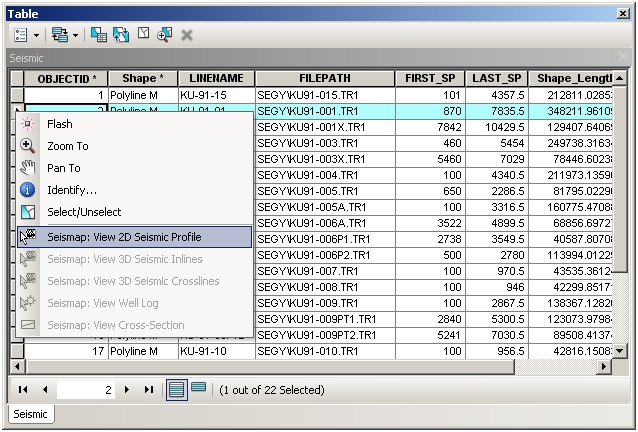
The image above shows the context menu for the Attribute Table of a 2D seismic layer (note - additional ESRI context menu items removed from image for clarity)
4.1 2D Seismic Layer Properties
2D seismic profiles can be displayed for measured polyline feature classes. Seismap layer properties can be accessed as a tab in the standard Layer Properties dialog.
Use this layer for Lynx Seismap 2D seismic (checkbox) - check this box to activate Seismap for this layer and enable the rest of the parameters on this property page.
Filepath Field - select the attribute table field which contains the path of the SEG-Y file. This field must be a string field, and should contain the path to the seismic data file for each seismic profile (feature). File paths are resolved in a similar way to that used for standard ArcMap hyperlinks - see File name resolution (below) for more information. To use the basemap labelling, export and intersection functionality of Seismap without any seismic data files to display, select the <No Filepath Field> option from the dropdown list.
SP Source - select Seismic File Header or
Attribute Table.
For 2D seismic data, the shotpoint range of the seismic data file, and the measure values of the 2D seismic
feature class, are used to show the current display range on the map, and mark intersections in the seismic
viewer windows. If the shotpoint range is not stored in the seismic data file, then ranges and intersections
will be incorrectly displayed.
- Seismic File Header - the first shotpoint and shotpoint increment are read from the seismic file header. Use this option for Lynx Trace files (TR files) and Lynx-variant SEG-Y data, which store these values in un-used slots in the binary file header. Standard SEG-Y contains no information on the exact shotpoint range (although integer shotpoint values may be stored in each trace header). SEG-Y Revision 1 files should contain decimal shotpoint numbers - see Import 2D Seismic Data for how to read these values.
- Attribute Table - for SEG-Y data (both standard and Revision-1) which does not contain shotpoint information in the file header, the first and last shotpoint values can be read from fields in the basemap layer's attribute table.
The following 2 parameters are only displayed if SP Source (above) is set to Attribute Table. For seismic data stored as SEG-Y format, there may be no shotpoint information available from the file itself. These parameters allow you to read shotpoint values from the feature class attribute table.
First Shotpoint Field - Select the field from this 2D Seismic Layer attribute table which contains the shotpoint value for the first trace of each seismic profile.
Last Shotpoint Field - Select the field from this 2D Seismic Layer attribute table which contains the shotpoint value for the last trace of each seismic profile.
Show Line Intersections (checkbox) - Indicate whether to display intersections with other lines in the shotpoint scale bar of seismic viewer windows.
Highlight Current SP Range on Map (checkbox) - Indicate whether to highlight viewer window shotpoint/CDP ranges on the map. The current range is interactive - you can use the 'hand' tool on the Seismap toolbar to grab and pan a displayed range in ArcMap's data view.
Highlight Colour - Select a colour for the current shotpoint/CDP range highlight
Highlight Width (px) - Set the width in pixels for the current shotpoint range highlight.
Line Name and SP Labels - click this button to access the simplified line and shotpoint labelling options for 2D seismic data. The options on this page can all be set within ArcMap using the 'Labels' and 'Hatches' tabs in the Layer Properties dialogue accessed by right-clicking on a layer in the ArcMap Table of Contents. However, for infrequent users, these options are often hard to find and obscure to set. The parameters as presented here provide a simpler interface to labelling which is specific to seismic shotpoint maps. These options do not provide a comprehensive alternative interface to ArcMap's hatch annotation options, but rather a 'quick and dirty' way to display annotation which can be fine-tuned later using the existing ArcMap interface.
Show Line Names (checkbox) - Indicate whether to display line name labels on the map using the options below.
Line Name Field - Select the line name field from the basemap layer attribute table from the drop-down list. This is usually the same as the layer's primary display field used for map tips.
- Start - line name labels will be placed before the start of the line
- End - line name labels will be placed after the end of the line
- Both - line name labels will be placed both before the start and after the end of the line
Line name labels will be oriented along the direction of the line. A bug in ArcMap means that text labels are never plotted 'upside-down' - ArcMap will always rotate text labels to what it considers a 'correct' orientation. This is contrary to conventions for seismic basemaps.
Line Name Font - Select the font to use for the line name labels. You will get best results using a true-type font.
Show SP Annotation (checkbox) - Indicate whether to display shotpoint markers on seismic profiles.
SP Nodes at Ends (checkbox) - Indicate whether to display shotpoint markers at the start and end of each seismic profile.
SP Node Interval - Specify an integer value as the interval between shotpoint markers. Markers will be placed where the shotpoint value is a multiple of this interval.
SP Node Symbol Size - Specify the diameter in points (approx 1/72 inch) of the shotpoint marker symbol.
SP Node Symbol Colour - Select the colour for
shotpoint marker symbols.
Seismap will only create coloured circles as
shotpoint markers. To use more complex symbols you can use the ArcMap Hatch Annotation
interface accessible by right-clicking the basemap layer in the ArcMap Table of Contents,
and selecting Properties.
SP Labels at Ends (checkbox) - Indicate whether to display shotpoint values as labels at the start and end of each seismic profile.
SP Label Interval - Specify an integer value as the interval between shotpoint labels. Labels will be placed where the shotpoint value is a multiple of this interval. The SP label interval is usually a multiple of the SP node interval, so that, for example, markers are placed every 10 shotpoints, and labels are placed every 50 shotpoints.
SP Label Decimal Places - Specify the number of decimal places that will be displayed for shotpoint labels. The default is 0, meaning that SP labels will be rounded to the nearest integer.
SP Label Font - Select the font to use for the shotpoint value labels. You will get best results using a true-type font.
Shotpoint labels will be displayed perpendicular to the line direction. A bug in ArcMap means that text labels are never plotted 'upside-down' - ArcMap will always rotate text labels to what it considers a 'correct' orientation. This is contrary to conventions for seismic basemaps.
Scale Range for Labels (checkbox) - Indicate whether to use the minimum and maximum scales below for line name and shotpoint labels and shotpoint markers.
Minimum Scale - Set a minimum scale for labels and markers. If you zoom out beyond this scale, labels and markers will not be displayed.
Maximum Scale - Set a maximum scale for labels and markers. If you zoom in beyond this scale, labels and markers will not be displayed.
Export iSeisview shapefiles - export this layer as shapefiles in the format used by Lynx iSeisview.
Select an output shapefile for the 2D seismic metadata table, and, if horizon overlays exist in this MXD, an output shapefile for horizons. If these output shapefiles already exist they will be overwritten. Features will be re-projected to WGS-84. Relative file paths to SEGY files will be used, as in this source layer.
Export to ASCII - export the current polyline-M layer as a UKOOA/SEG-P1 or CSV format ASCII file.
You can select the following export formats from the standard Save File dialogue:
- Comma-delimited text (CSV) - CSV output files created by Seismap will always use a comma as the field separator and a period as the decimal separator, regardless of the regional settings on your PC. If you have problems opening a CSV file with Microsoft Excel, because it is expecting a different field separator character, use the Data-Get External Data-Import Text File menu option, which displays a wizard allowing you to specify the delimiter and decimal separator to use.
- UKOOA text - a text file formatted approximately according to the UKOOA/SEG-P1 standard.
Features will be exported using the coordinate system of the underlying feature class, rather than the current display coordinate system. If the output filename you specify already exists, it will be overwritten.
4.2 3D Seismic Layer Properties
3D seismic inlines and crosslines can be displayed for 4-dimensional polygon feature classes (coordinate values must contain either X,Y,Z,M or X,Y,ID,M values)
Use this layer for Lynx Seismap 3D seismic (checkbox) - check this box to activate Seismap for this layer and enable the rest of the parameters on this property page.
Polygon Attributes - select from
ID=Inline M=Xline or Z=Inline M=Xline
Seismap uses
polygons to store the outlines of 3D seismic surveys. The inline and crossline
numbers are stored at each polygon vertex. Locations of intermediate CDPs are
calculated on the fly by using a Delaunay triangulation, thus reducing the size
of the polygon feature class required for display by ArcMap.
Polygon outlines can be generated for 3D surveys from CDP coordinates or inline
polylines using the Import 3D Seismic Data wizard for
ArcMap.
There are 2 different ways in which the inline and crossline numbers
in each polygon vertex can be stored, depending on the underlying format of the
feature class:
- ID=Inline M=Xline - the inline number is read from each point's ID and the crossline number from each point's measure value. Use this option when the polygon layer is in a geodatabase. This is the best way to store the 3D grid information, since it does not misuse the Z (height) coordinate value, however it is not compatible with shape files.
- Z=Inline M=Xline - the inline number will be read from the Z coordinate value, and the crossline number from the measure value. Use this option when the polygon layer is a shape file, since shape files do not support point IDs.
Filepath Field - Select the attribute table field which
contains the path of the 3D SEG-Y file. This field must be a string field and should contain
the path to the seismic data file for each 3D seismic survey (feature).
The seismic data should be stored in a single SEG-Y file per survey, sequential inlines stored end-to-end,
with ascending crossline numbers for each inline. It is not necessary to pad all inlines to the same number of traces.
Ideally, inline and crossline numbers should be stored in standard trace header slots, but if different 3D surveys
have the information in different header slots, this can be handled below
File paths are resolved in a similar way to that used for standard ArcMap document hyperlinks, and can be
absolute or relative,
and can include environment variables.
Inline/Xline byte locations - select from Fixed, Attribute Table
or SEG-Y Revision-1
Specify how to read the inline and crossline numbers from the seismic data files.
Each seismic survey must only use one seismic data file, but you may have more than
one seismic survey outline in your 3D seismic layer, and thus more than one seismic data files,
with incompatible header slots for inline and crossline numbers.
All methods assume that the inline and crossline are stored as 4-byte big-endian (non-Intel) order integers.
- Fixed - select this option if all your seismic data files use the same header slots to define inline and crossline numbers, and define the trace header slots below.
- Attribute Table - select this option if your seismic data files use different header slots to define inline and crossline numbers. The inline and crossline header slots for each seismic data file can be read from fields in the feature class attribute table - define the fields to use below.
- SEG-Y Revision-1 - select this option if your seismic data files conform to the SEG-Y Revision-1 standard, which specifies that the inline number is stored in trace header bytes 189-192, and crossline is stored in bytes 193-196.
Inline Header Byte
Xline Header Byte
For Fixed header slots (above), select the (1-based) trace
header starting byte from which to read the inline and crossline numbers for each trace.
Note that the value must be a 4-byte integer. The values specified here must be aligned on a 2-byte
or 4-byte boundary (ie, they must be odd numbers).
Inline Header Field
Xline Header Field
For Attribute Table header slots
(above), select the fields from which to read the inline and crossline header
slots.The fields used must be of type Integer or Small Integer.
The fields should contain the 1-based starting byte of the header slot to use.
Highlight Current Trace Range on Map (checkbox) - Indicate whether
to highlight viewer window trace ranges on the map. The current range is interactive - you can use
the 'hand' tool on the Lynx Seismap toolbar
to grab and pan a displayed range in ArcMap's data view.
Highlight Colour - Select a colour for the current trace range highlight
Highlight Width (px) - Set the width in pixels for the current trace range highlight.
Export...
Export iSeisview shapefile - export this layer as shapefiles in the format used by Lynx iSeisview.
Select an output shapefile for the 3D seismic metadata table. If this output shapefile already exists it will be overwritten. Features will be re-projected to WGS-84. Relative file paths to SEGY files will be used, as in this source layer.
4.3 Seismic Viewer Window
Each seismic viewer window displays a 2D seismic profile or a 3D inline
or crossline.
Multiple windows can be open viewing different profiles at the
same time.
The shotpoint/CDP range currently displayed will be superimposed
on the 2D line or 3D survey in ArcMap's data view.
The Seismic Display parameters allow you to set display and scale
parameters globally for all 2D and 3D seismic viewer windows. Changes made here
will be applied to all currently open and subsequently open seismic viewer
windows. These parameters are accessed via the
Seismic Display Options
menu on the Seismap toolbar and the Options-Display Properties
menu item in seismic viewer windows.
Parameters are displayed in a wizard-style PRMEDIT dialogue.
Seismic Display Style and Scale Page
This parameter page allows you to set the display style, scale and amplitude for seismic displays.
Display Style
Select the trace display type:
- VA Variable area only
- Wiggle Wiggle trace only
- VA/Wiggle Variable area with wiggle trace overlay
- Greyscale Sample Greyscale black (high amplitude) to white (low amplitude) variable density sample display
- Blue-White-Red Sample Blue (high amplitude) to white to red (low amplitude) sample display
- Blue-White-Red Sample/Wiggle Blue to white to red colour sample display with wiggle trace overlay
- Greyscale Interpolated Greyscale black (high amplitude) to white (low amplitude) variable density subsampled to individual pixels
- Blue-White-Red Interpolated Blue (high amplitude) to white to red (low amplitude) display sub-sampled to individual pixels
- Orange-White-Black Interpolated Orange (high amplitude) to white to black (low amplitude) display sub-sampled to individual pixels
- Green-White-Brown Interpolated Green (high amplitude) to white to brown (low amplitude) display sub-sampled to individual pixels
Horizontal Scale
The approximate horizontal trace scale ratio for initial display
and full-scale plotting, eg 1:25000 will give a 1mm trace spacing if the input trace file has a CDP spacing of 25m.
For trace files where the trace spacing is unknown, a default value of 25m is assumed. The trace spacing is read from the
seismic file header. In Lynx TR-files and Lynx-variant SEG-Y files the trace spacing is read from a known header slot,
however, the trace spacing is not stored in standard SEG-Y files, so the default value of 25m will be used.
Vertical Scale
The approximate vertical scale, used for initial display on-screen
and full-scale plotting.
Vertical Scale Units
Select the units used for the vertical scale:
either cm/sec or inches/sec.
The horizontal and vertical scales set here determine the intial scale at which seismic profiles are displayed.
You can zoom in and out from this scale using the various zooming options available from the seismic viewer
window menu and toolbar. You can return to this initial scale using the Zoom to Preset Scale
 option. This initial scale is also the scale used for printing
full-scale seismic plots using the Print
option. This initial scale is also the scale used for printing
full-scale seismic plots using the Print  option.
Amplitude Factor
The amplitude factor f is calculated relative to RMS,
the root mean square amplitude for the input data traces. The display amplitude is adjusted so that
RMS = 3 x trace spacing and then multiplied by f. Setting f = 1.0 should give a reasonable looking
VA/Wiggle display. Colour and greyscale displays are such that 3 x RMS is equal to the maximum range
of the palette. Setting f to greater than 1.0 will increase the saturation and may cause clipping.
Why three times? - because the peak-to-peak amplitude of normally distributed samples will be approx 2 root 2, or 2.828
times the RMS. That's near enough 3, to geophysical accuracy.
- Auto - the RMS amplitude of the input data will be calculated and used in the amplitude factor calculation above. Most of the time, this will work quite well.
- Fixed - a fixed input amplitude will used to scale the data. This amplitude shoud be entered below.
Peak Amplitude
Enter the amplitude value to correspond with one trace spacing
(VA or Wiggle displays), or to the maximum range of the palette (greyscale or colour display)
Seismic Display Units Page
This parameter page allows you to specify the units used on the seismic display windows.
Upper Trace Scale
Select from: None, Trace, CDP, Shotpoint, Distance
Type of scale used for the upper scale bar, above the trace display.
The scale-type chosen here will also be used to show the current X mouse-position in the status bar when the
mouse is moved over the viewer window.
Note: for 3D seismic viewer windows, selecting shotpoint will display the inline or crossline numbers.
Upper Trace Scale Units
Select the units for the upper trace scale (only activated when the upper trace scale is Distance)
Lower Trace Scale
Select from: None, Trace, CDP, Shotpoint, Distance
Type of scale used for the lower scale bar, above the trace display
Note: for 3D seismic viewer windows, selecting shotpoint will display the inline or crossline numbers.
Lower Trace Scale Units
Select the distance units for the lower trace scale
(only activated when the lower trace scale type is Distance)
Line and well intersections (see Basemap Layer Options (above)) will be displayed in either the upper or lower trace scale if the type is set to Shotpoint.
Left Scale Units
Select from: msecs, microsecs, secs, samples)
Type of scale used for the vertical left time scale bar. The scale-type chosen here will also
be used to show the current Y mouse-position in the status bar when the mouse is moved over the viewer window.
Right scale Units
Select from: msecs, microsecs, secs, samples
Type of scale used for the vertical right time scale bar.
Seismic Display Grid Page
This parameter page allows you to specify grid lines to overlay the seismic display. This is often useful for full-scale plots.
Show Timing Lines - YES/NO
Indicate whether to display horizontal timing lines on seismic displays.
Timing Line Interval, msec
Specify the interval in msec for the timing lines
Show Trace Lines - YES/NO
Indicate whether to display vertical trace lines on seismic displays.
Trace Line Interval, traces
Specify the interval in traces for the trace lines.
Line Colour
Select the colour for the timing lines and/or trace lines.
The seismic viewer window uses standard Lynx Viewer component menus and toolbar buttons which allow you to zoom in and out, compress horizontally or vertically, flip the display, and print the profile, which are described in detail in Viewer Common Functionality. and Seismic 3D Inline Display.
In addition to the standard viewer toolbars, the seismic viewer window also has a toolbar containing tools specific to Seismap - the Identify Toolbar - which has the following tools:
Identify  - view the feature attributes for the current
2D profile, 3D survey, or well formation top when the mouse is clicked on the viewer window, in a standard ArcMap Identify
dialogue.
- view the feature attributes for the current
2D profile, 3D survey, or well formation top when the mouse is clicked on the viewer window, in a standard ArcMap Identify
dialogue.
Open Intersection - for 2D profiles or well intersections,
click on an intersection label in the shotpoints scalebar to open the intersecting seismic
profile or wireline well log. For 3D profiles, click anywhere in the inline/crossline scalebar
to open the intersecting inline/crossline at the current location.
2D Profiles
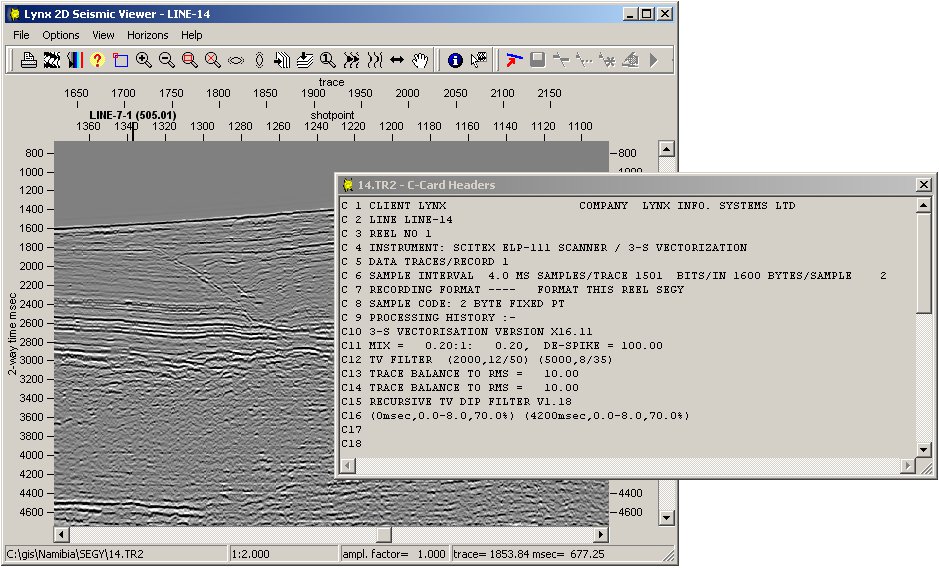
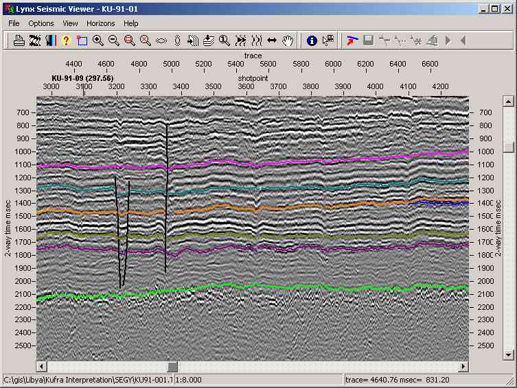
The image above shows a 2D seismic viewer window in Greyscale display mode with line intersections and the C-Card header display.
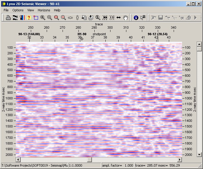
The image above shows a seismic viewer window in Interpolated Colour display mode with line and well intersections.
3D Inlines and Crosslines
For details of the additional options available for viewing 3D seismic data, see Seismic 3D Inline Display
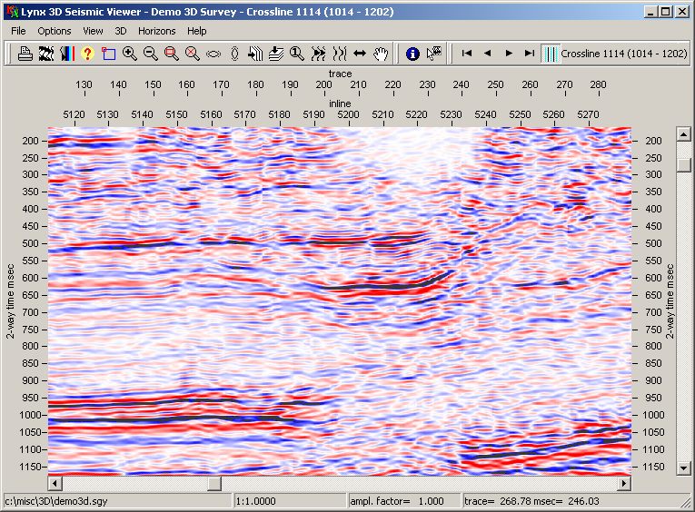
The image above shows a 3D crossline in Interpolated Colour mode. The 3D seismic viewer window has an extra toolbar showing the current inline/crossline number, and allowing you to browse between profiles.
4.4 Import 2D Seismic Locations
You can convert a UKOOA/SEG-P1 file or CSV file containing shotpoint/CDP
coordinates into a file geodatabase feature class or shape file using the
Lynx Seismap toolbar menu option Import/Export - Import Seismic Locations.
This uses the Lynx utility UKO2SHP. For more information about converting
UKOOA/CSV files, see the help for UKO2SHP. After you
have converted your input file, you will be prompted to select a spatial
reference for the generated feature class. This feature class will be added to the
current ArcMap data frame.
In order to use the feature class created here as a 2D seismic basemap layer in Seismap,
you will need to import 2D seismic data using the option below,
or add a field to the attribute table and edit seismic data filepaths into this
field.
Metadata will automatically be created for the generated feature class, listing the import process. Only FGDC format metadata is supported in this version. To turn off generation of metadata by Seismap, edit the import metadata key in the [startup] section of the seismap.ini file to be a blank value.
4.5 Import 2D Seismic Data
Seismap reads seismic data in its pre-existing SEG-Y format or Lynx Trace file format - there is no need to reformat the seismic data files. The seismic 2D import wizard displayed by the Import 2D Seismic Data menu provides a simple method of importing seismic data, but you can also use standard ArcGIS Desktop functionality to create and edit existing layers.
The wizard provides a choice of output layer types: you can create a route event using a seismic list in a standalone File Geodatabase or dBASE table, or a new feature class in a File Geodatabase or shapefile.
Before using this wizard, you must already have the seismic locations loaded as a layer in the current ArcMap data frame (see Import 2D Seismic Locations). The wizard provides visual confirmation that the line-names of your seismic data files match your existing seismic locations layer, but you should verify independently that shotpoint ranges in your seismic data files match those in your seismic locations. For more advanced reconciliation tools, see the Lynx Seismatch application.
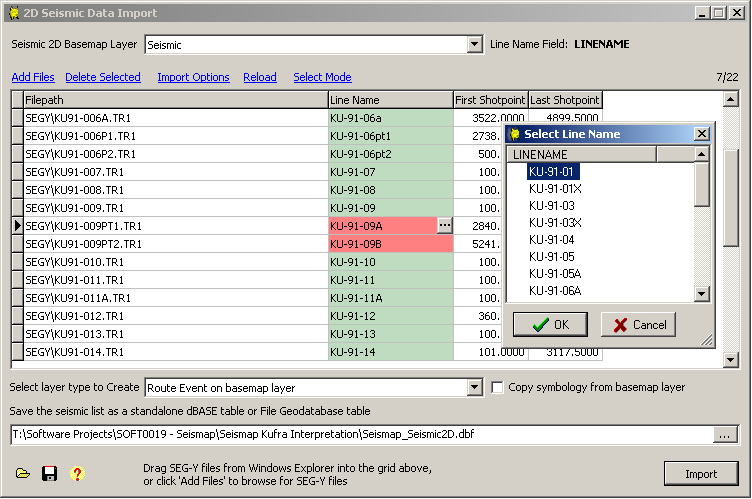
Import 2D Seismic wizard, showing relative file paths and line-name pick-list
First, select your seismic 2D locations layer from the drop-down list. Select from all available polyline-M layers in the current map data frame
The Import 2D Seismic Options determine how the required information is read from the listed SEG-Y files.
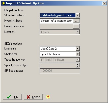
File path options
Select whether to store seismic file paths as absolute, relative or using an
environment variable. If you choose to use relative paths, you must specify the base
folder from which these relative paths will be resolved. This will be saved as the Hyperlink Base
in your MXD. If you choose to use an environment variable, select whether to use $- or %-notation - there
are advantages and disadvantages to both. For more discussion of these options, see
File name resolution (below).
SEG-Y options
Select how to read linename and shotpoint information from the seismic data files.
The linename is conventionally stored in C-Card 2, but alternatively, you can use the filename.
For Seismap to work correctly, you must ensure that the linename here exactly matches
the linename in the seismic locations layer, so some manual editing may be
necessary.
You can choose to read the shotpoint range from the Lynx
binary file header (this is the most reliable method, but only works for Lynx
trace files and Lynx-variant SEG-Y) or from a specified slot in the first and
last trace headers. A number of pre-defined slots are defined for various SEG-Y flavours,
or you can select a custom header slot to read a 4-byte integer shotpoint number. Note that
shotpoint numbers in trace headers are likely to be approximate - the original SEG-Y (Revision 0)
format specification was slightly vague on shotpoint numbers; SEG-Y Revision 1 formatted files
will have accurate (scaled integer) shotpoint numbers in trace headers).
Next, drag SEG-Y files from an Explorer window onto the wizard window,
or click Add Files to browse for SEG-Y files. Each selected file will be added to the displayed list.
Click Delete Selected to remove selected records from the list.
Click Import Options to edit the Import 2D Seismic Options (see above).
Click Refresh to re-read filepaths, linenames and shotpoint ranges from the seismic files using the current import options.
Click Edit Mode/Select Mode to switch between row-select mode, which allows you to select multiple records for deletion,
and field-edit mode, which allows you to manually edit field values in the list.
The line name for each SEG-Y file will be highlighted in red or green. A red highlight means the line name is not present in the selected seismic 2D basemap layer. Click the '...' button in the linename field when in Edit Mode (or press Ctrl+Enter) to display the linename picklist to select the correct linename from your seismic 2D basemap layer. Linenames often differ in spacing or capitalisation - you must ensure that line names match exactly for the table relationships created by Arcmap to function correctly. A green highlight means the line name is present in your selected seismic 2D basemap layer.
The buttons at the bottom of the wizard window allow you to save and reload the displayed list of SEGY files:
 - load an existing dBASE (DBF) file saved in this wizard.
 - save the current list as a dBASE (DBF) file.
 - display this help.
Choose the type of layer to create - either a new route event layer or a new feature class:
- Route Event - your list is saved as a standalone table in a File Geodatabase or in dBASE format. This list is then added to your current ArcMap data frame as a new route event layer, using the line-names to match features in your selected seismic 2D basemap layer, and the first and last shotpoints as linear referencing on the basemap layer polyline measures.
- New Feature Class - stored in a File Geodatabase or as a shapefile. This option creates a new feature class layer containing a copy of the line geometry for each matched line from your selected seismic 2D basemap layer. This new layer is then added to your current ArcMap data frame.
For either of these options, it is important that the line names in your seismic list match the line names in your seismic 2D basemap layer.
You can choose to copy the symbology of your basemap layer to your newly created layer by ticking the Copy Symbology checkbox.
Select a name and output location: for route event output, you will be creating a standalone table in a File Geodatabase or in dBASE format; for new feature class output, select a File Geodatabase and specify a new name, or create a new shapefile.
Click Import to save your seismic list, create the layer, and set the Seismap layer properties for this new layer. You can then activate the Select Seismic Profile tool and view your SEG-Y files
4.6 Import 3D Seismic Data
Seismap uses polygons to define 3D seismic surveys.
Using the Import 3D Seismic Data Wizard, Seismap can read trace coordinate values from trace headers in 3D seismic SEG-Y files, to generate the survey outline polygons.
Each seismic survey is defined as a single polygon feature. Inline and crossline numbers are defined at each of the polygon vertices. Locations of intermediate CDPs are calculated on the fly by using a Delaunay triangulation, thus reducing the size of the polygon feature class required for display by ArcMap.
A single polygon layer may store the locations for multiple 3D seismic surveys.
The underlying format of the feature class determines whether the inline and crossline numbers are stored in each point's ID and M (geodatabase feature classes) or Z and M (shape files).
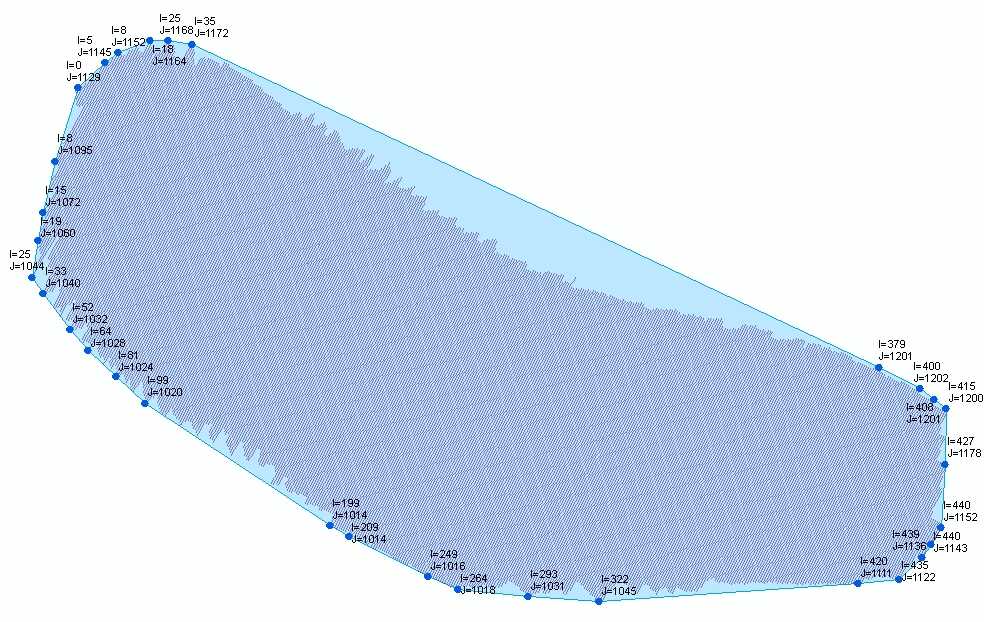
This image shows:
- The original live traces, stored as one polyline per inline with the crossline numbers as measures
- The generated convex hull polygon
- For illustrative purposes, each vertex of the polygon is labelled with its inline (I) and crossline (J) numbers.
3D Survey Import Wizard
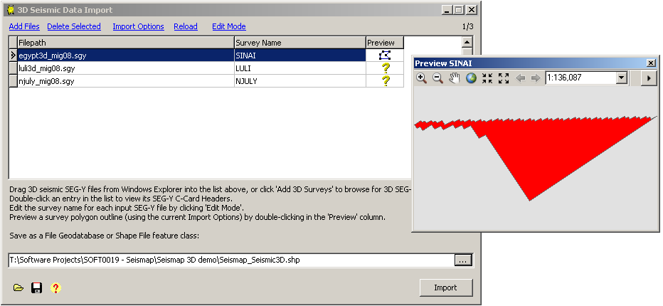
Import 3D Seismic wizard, showing relative file paths, edited survey names and a survey outline preview
Drag 3D seismic SEG-Y files from an Explorer window onto the wizard window,
or click Add 3D Surveys to browse for SEG-Y files. Each selected file will be added to the displayed list.
Click Delete Selected to remove selected records from the list.
Click Import Options to edit the Import 3D Seismic Options (see below).
Click Refresh to re-read filepaths from the seismic files using the current import options.
Click Edit Mode/Select Mode to switch between row-select mode, which allows you to select multiple records for deletion,
and field-edit mode, which allows you to manually edit field values in the list.
You can double-click in the Filepath column to view the C-Card headers for the selected file, or in the Preview column to preview the survey outline for selected file using the current Import Options (see below). Note that previewing a large SEG-Y file involves reading all trace headers - this may take some time.
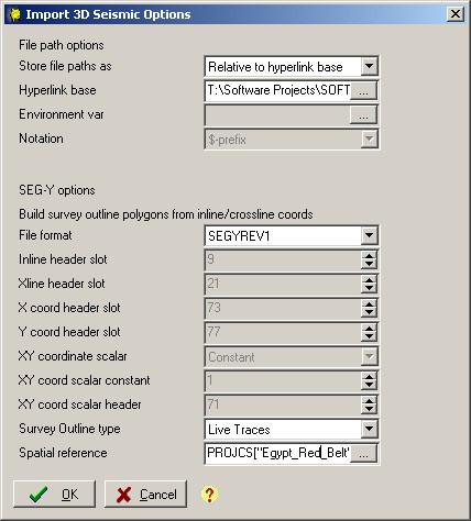
The Import 3D Seismic Options determine how the required information is read from the listed SEG-Y files.
File path options
Select whether to store seismic file paths as absolute, relative or using an
environment variable. If you choose to use relative paths, you must specify the base
folder from which these relative paths will be resolved. This will be saved as the Hyperlink Base
in your MXD. If you choose to use an environment variable, select whether to use $- or %-notation - there
are advantages and disadvantages to both. For more discussion of these options, see
File name resolution (below).
SEG-Y options
Select how to read inline/crossline/coordinate values from the trace headers, and the type of survey outline
polygon to generate.
Choose from SEGY or SEGYREV1 file formats - SEGYREV1 is a well-defined format which specifies
exactly in which trace headers the inline/crossline numbers and coordinate values are stored - most modern 3D
seismic data files are stored in SEGYREV1 format:
| Name | Trace Header Bytes |
|---|---|
| Inline number | 189-192 |
| Crossline number | 193-196 |
| X coordinate | 181-184 |
| Y coordinate | 185-188 |
| XY coordinate scalar | 71-72 |
If the input files are not SEGYREV1, then you will have to specify which trace headers contain the inline/crossline numbers and XY coordinates. Sometimes this information is written as comments in the SEG-Y C-Card header - double click the row in the list to view the C-Cards for the selected SEG-Y file.
Seismap can generate three different levels of survey outline polygon of increasing complexity. You can choose whether to output a Rectangle of inline/crossline minima/maxima, a Convex Hull outline of live traces, or a Live Traces polygon.
You must also specify the spatial reference used by the coordinates in the input SEG-Y files. This is required for the feature class generation. By default, this spatial reference parameter is initialised to the spatial reference of your current active data frame in ArcMap.
Once your import parameters are set and you have added your 3D seismic survey SEG-Y files and edited their survey names, select an output polygon feature class to create - you can choose to create either a polygon shapefile or a polygon feature class in a file geodatabase. If you choose a feature class which already exists, it will be overwritten.
The buttons at the bottom of the wizard window allow you to save and reload the displayed list of SEGY files:
- - load an existing dBASE (DBF) file saved in this wizard.
- - save the current list as a dBASE (DBF) file.
- - display this help.
Click the Import button - a dialog will be displayed showing your current import options, click OK to start the
import process.
3D seismic survey SEG-Y files are very large, and this import process may take a considerable amount of time -
10 to 30 minutes would not be unusual.
When the import process is complete, the generated polygon feature class will be added to your active data frame in ArcMap, and initialised as a Seismap 3D seismic layer.
Note that this initial import implementation builds the inline and crossline index files for each seismic survey used for fast display of inlines and crosslines in the seismic viewer. These index files are stored on your local PC in your Lynx CUSTOM folder (see Cached Seismic Data for details). These indexes will be regenerated automatically if they do not exist, but this can take some time, and may delay the initial display of inlines/crosslines. If you intend to access this MXD from multiple PCs, then you can move these inline and crossline index files into the same folder as the SEG-Y files - this will avoid these index files being recreated locally on each PC or for each user.
4.7 Cached Seismic Data
Seismap stores 2D profile, horizon and well intersection information after its initial calculation for quick retrieval. This information is stored in the MXD along with other Seismap parameters. Seismap also creates inline and crossline index files for 3D seismic volumes when a 3D seismic data file is first opened, which speeds up subsequent displays of the same file - these index files are stored in your Lynx CUSTOM folder. If you change inline or crossline header information, or if you edit geometries manually, this cached information may become out of date, and cause Seismap to display data incorrectly. The Cache Management option on the Seismap toolbar menu can be used to delete this cached information, so that intersections and index files will be recreated the next time a seismic file is displayed.
5. Seismic Horizons, Surfaces and Faults
- 5.1 Horizon and Fault Layer Properties
- 5.2 Horizon Z-Value Colour Ramp Renderer
- 5.3 Horizon/Fault Import and Export
- 5.4 Horizon/Fault Polyline Export
- 5.5 Horizon/Fault Polyline Import
- 5.6 Grid Import and Export
- 5.7 Exporting a Z-Map Grid
- 5.8 Importing a Z-Map Grid
Lynx Seismap can display polylines with Z values, as well as TIN and raster grid surfaces, as horizon and fault overlays on 2D and 3D seismic profiles.
The image above shows horizon and fault overlays on a Greyscale trace display.
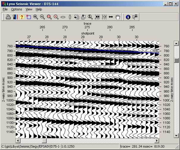
The image above shows a horizon overlay on a VA-wiggle trace display.
5.1 Horizon and Fault Layer Properties
The polyline layers or surfaces must be listed in the current document in ArcMap, as part of the same data frame as the 2D and/or 3D seismic basemap layer. To display TIN surfaces you must have the 3D Analyst extension installed and licensed. To display polyline-Z layers or raster grid surfaces no extra licence is necessary. The polylines or surfaces must be attributed with Z-values in two-way-time in milliseconds (to match the seismic data vertical scale), as depth-to-time conversion using velocity data is not yet implemented. Polyline feature classes used for horizon/fault overlay must include a primary display field which uses the same line names as the corresponding 2D seismic layer. Seismap layer properties can be accessed as a tab in the standard Layer Properties dialog.
Show as Horizon/Fault Overlay on 2D and 3D Seismic (checkbox) - activate horizon fault overlay for this layer, and enable the rest of the parameters on this property page.
Display as - select from Horizon or Fault
Display Colour - select colour for horizon overlay on seismic profiles.
Display Width - select pixel width for horizon overlay on seismic profiles.
Visible (checkbox) - show/hide the horizon/fault seismic overlay independently of the layer's visibility in the ArcMap map view.
Depth Units - select TWT (ms) two-way time in milliseconds. Depth units of the horizon layer must be in ms. Depth-to-time conversion is not yet implemented.
Export - click this button to export the horizon/fault in a variety of ASCII formats - see below.
The drawing order of horizons and faults as seismic overlays will be the same as the display order listed in ArcMap's table of contents view - the last horizon/fault listed is drawn first - later horizons will overlay earlier ones.
5.2 Horizon Z-Value Colour Ramp Renderer
Seismap includes a custom feature renderer to display horizon and fault polylines by their Z value with a user-specified colour ramp.
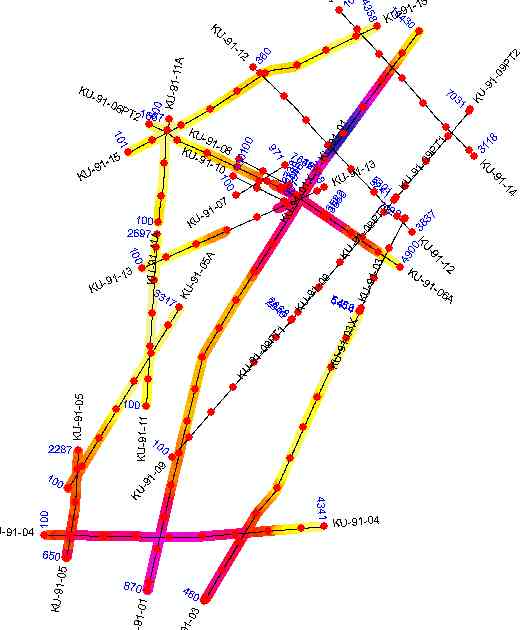
The image above shows a horizon polyline layer displayed using the Z-value colour ramp renderer, with a shotpoint basemap.
The settings for this custom renderer can be accessed on the Symbology tab in the Layer Properties dialog.
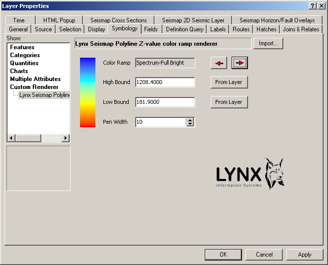
You can use the arrow buttons to browse backwards and forwards through the standard colour ramps from the ESRI Style Manager. The 'From Layer' buttons can be used to set the upper and lower Z values for calculating the corresponding colour for each intermediate Z value. Z values outside the bounds entered here will be displayed with the high-bound or low-bound colour.
This polyline-Z colour ramp symbology can be saved into layer files and previewed in ArcCatalog; however, ArcScene and ArcGlobe are not supported.
5.3 Horizon/Fault Import and Export
Seismap provides import and export options for interpreted horizon and fault picks.
Seismic interpretation systems provide a number of export formats for horizons and faults. The import options in Seismap are flexible enough to deal with many different formats exported from seismic interpretation systems or digitising applications, using a spreadsheet-like (CSV or column-delimited) layout or shapefile, as long as they contain at least the following information:
- Linename
- Shotpoint
- X coordinate (can be interpolated from existing seismic line locations if not present)
- Y coordinate (can be interpolated from existing seismic line locations if not present)
- Z-value (TWT in seconds or milliseconds)
- In addition, the format must contain some method of separating line segments - either with a segment identifier, or with null-value records in between each segment.
The recommended export formats for picked horizons and faults from IHS Kingdom are as follows:
2D Horizons
The full range of each interpreted line is output, with null values marking breaks/discontinuities,
allowing horizons to be imported as multi-part polylines with X and Y, plus Z
as TWT and M as SP.
Note that these export formats will not handle
reverse-faulted horizon segments or overthrust horizon segments.
Use either of the following export formats from Kingdom:
Landmark Time
Ensure the 'with nulls' checkbox is ticked. This will generate a column-delimited ASCII text file containing records in the following format:
LINENAME SP X Y Z
Z-values are TWT in millisecondsLine Trace X Y Time
Ensure the 'with nulls' checkbox is ticked. This will generate a comma-delimited ASCII text file containing records in the following format:
LINENAME,SP,X,Y,Z
Z-values are TWT in seconds
2D Faults
Fault segments can be exported from Kingdom using Charisma format, which uses a record format
with an arbitrary segment ID for each separate fault segment in the following
format:
LINENAME SP X Y Z FAULTNAME ID LINENAME
5.4 Export Horizon/Fault Polylines
You can export horizon/fault layers from Seismap using the Export to ASCII button on the 'Seismap Horizon/Fault Overlay' tab page of the Layer Properties dialog. These exported files can be imported into SMT Kingdom, Landmark, or other seismic interpretation systems.
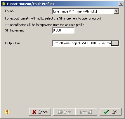
Select the horizon/fault and export format from the drop-down lists. The formats currently supported for horizon/fault export are:
- Line Trace X Y Time (with nulls) - Z-values will be converted from milliseconds to seconds. Comma-delimited output
- Landmark Time (with nulls) - Z-values will be output as-is - assumes milliseconds. Column-delimited output
- Charisma (faults). Column-delimited output
- Custom - see below
Set the output shotpoint increment for lateral sampling of the horizon. This is only applicable for the 'Line Trace X Y Time' and 'Landmark Time' formats, which separate segments with null values. You should select a shotpoint increment value which will output a value for each trace in the seismic data.
If you select the Custom format option, the next page of the export wizard will allow you to specify how to write your output file, by specifying the field order. Use the 'Segments Separated By: Null Values/Segment ID' option to determine the type of line-part separator in your output file, and select the output units for the Z-value.
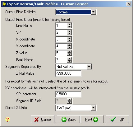
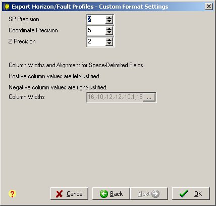
For Custom formats, you will also need to specify the precision used to write shotpoint, coordinate and Z-values. The precision is the number of decimal places used.
For space-delimited custom formats, you must also specify the column width and alignment for each output column. Enter the width for each in the list as shown. A positive width value implies that the column will be left-justified, and a negative width value implies that the column will be right-justified.
5.5 Import Horizon/Fault Polylines
You can import horizons and faults for any seismic lines in your seismic 2D basemap layers.
The import process can use linear referencing to create XYZM polyline features from your imported horizon shotpoint/TWT coordinates.
Your seismic locations must cover the full shotpoint range of your horizons, as no shotpoint extrapolation
is performed by this import operation.
The Import Horizon/Fault dialog is accessed from the Import/Export menu on the Seismap toolbar.
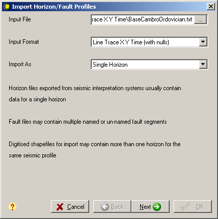
First page of Import Horizon/Fault Profile wizard
Select your input file and its format. The formats currently supported for horizon/fault import are:
- Line Trace X Y Time (with nulls)
- Landmark Time (with nulls)
- Charisma (faults)
- Custom Text Format - use a CSV or column-delimited ASCII file and specify the columns and segment separators to use
- XZ Shapefile - digitised horizon polylines saved in shapefile format using a pseudo-XZ coordinate system. Your digitised shapefile should be calibrated to use seismic shotpoints or distance along line as the X coordinate, and two-way time in msec as the Y coordinate. Your shapefile can contain a multi-part polyline feature for each digitised horizon/fault, or multiple features with the same feature name for a single horizon - these will be combined into a multi-part polyline. You can include different horizons in the same shapefile - a separate output shapefile will be created for each named horizon. Your shapefile must include attributes listing the HORIZON NAME and SEISMIC LINE NAME for each polyline.
The first 3 formats above are compatible with horizon/fault export options offered by IHS Kingdom.
Select 'Import As' Single Horizon or Multiple Horizons or Faults from the drop-down list. Horizons and faults are treated differently on import. When importing a horizon, the entire import file is assumed to refer to a single horizon, and so a single horizon feature class will be created. When importing faults, multiple named and un-named faults and fault-segments may be included in the same import file. so a separate feature class will be created for each named fault, and all unnamed fault segments will be added to an 'unassigned faults' feature class.
If you select the Custom format option, the next page of the import wizard will allow you to specify how to read your input file, by specifying the field order. The shotpoint field is optional - if it is not present in your input file, set this value to zero. Use the 'Segments Separated By: Null Values/Segment ID' option to determine the type of line-part separator in your input file, and select the units for the Z-value.
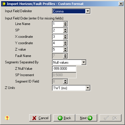
Custom format page of Import Horizon/Fault Profile wizard/p>
If you
select the XZ Shapefile format option, the next page of the import wizard will
allow you to define the measurement systems used for your input coordinates, and the
attribute fields used to retrieve the horizon name and seismic line name for each
horizon in your input shapefile.
Your input shapefile must contain an attribute naming the
seismic line for each feature (the seismic line names used here must match a line name
in one of your existing seismic 2D basemap layers). If your shapefile contains more than
1 horizon, you must also have an attribute naming the horizon. If you only have a single
horizon in your input file, you can use the name of the input shapefile as your horizon
name.
If you have multiple horizons with the same name in your input shapefile, these will be
combined into a single multi-part horizon polyline in the output feature class.
You can have horizons for multiple seismic lines and/or multiple horizons in the
same input file - separate output feature classes will be created for each horizon, containing
the horizon polylines for multiple seismic lines.
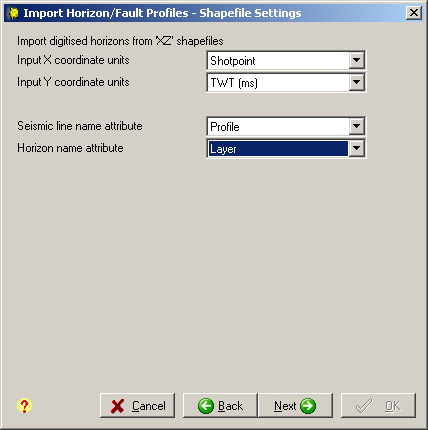
XZ Shapefile page of Import Horizon/Fault Profile wizard
On the final page of the wizard, select an output feature class
or destination folder/file geodatabase, and a spatial reference.
For single horizon import from a text file, select an output feature class in either file geodatabase format or
shapefile format.
For multiple horizon/fault import, select an output file geodatabase or folder - each named horizon/fault
in the input file will be stored as a separate feature class/shapefile in this output destination). If your destination
already contains feature classes, then you can tick the 'Add new features to existing feature classes' option
to merge your new features into these existing feature classes if the feature class names match your input horizon/fault names.
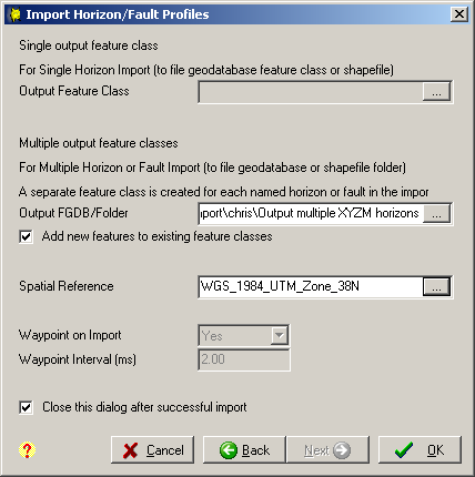
Final page of the Import Horizon/Fault Profile wizard
You can simplify the imported horizon/fault profiles by waypointing using a specified maximum vertical deviation in ms. This will create a much smaller feature class which will display more quickly in the seismic viewer windows. This option is only available for input from text file formats.
The 'Close this dialog after successful import' option allows you to import multiple text files easily, by reselecting a new input file if all other import parameters remain constant.
The import process will create a shapefile containing polyline-XYZM
features for each horizon import file, or a shapefile for each named horizon/fault in
the fault import file or XZ shapefile.
Z-values will be two-way time in ms, and M-values will
be shotpoint values (if present in the input ASCII file). The imported feature
class will be added to the Horizon/Fault list for display as a seismic
overlay.
The picked horizon/fault for each seismic profile will be stored as
a separate feature. The profile (seismic line) names used in the horizon layer
must match those used in a 2D seismic layer. Multi-part polylines allow
discontinuous horizons and reverse faults to be correctly represented. See
5. Horizons and Faults (above) for more
information on displaying overlays on seismic profiles.
5.6 Grid Import and Export
Seismap allows interchange between File Geodatabase Grids and ESRI Raster Grids and Z-Map ASCII grid files. ZMap is commonly used exchange format for gridded data such as seismic horizon and fault surfaces.
There are a few important differences between Z-Map and ESRI grid
formats.
Firstly, the Z-Map grid format allows independent grid sample
intervals in the X and Y directions, whereas an ESRI grid must have square
cells. Seismap will interpolate the grid values if required, to
recalculate cell values using the smaller of the X or Y grid sample intervals.
Interpolation will result in a larger number of cells in the output ESRI
grid
Secondly, the limits of a Z-Map grid are defined by the coordinates of
the corner nodes, whereas the limits of an ESRI grid are extended by half a
grid cell size around the cell centroid.
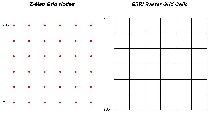
The diagram above displays the difference between the sample nodes used by Z-Map grids, and the sample cells used by ESRI grids.
5.7 Exporting a Z-Map Grid
You can export grid and TIN surfaces from Seismap using the Export to ZMAP Grid button on the 'Seismap Horizon/Fault Overlay' tab page of the Layer Properties dialog for grid and TIN surfaces. The output grid file will use the same spatial reference as the input surface layer. An output .dat file will be created in ZMAP ASCII Grid format.
5.8 Importing a Z-Map Grid
The Import ZMAP Grid dialog is accessed from the Import/Export menu on the Seismap toolbar.
Select the input Z-Map grid file, and specify an output name and path for the File Geodatabase grid or ESRI raster grid file (note that the standard restrictions apply to ESRI raster grid filenames - max 13 characters, no spaces etc). If the output grid already exists, you will be prompted to confirm overwriting it. Select the spatial reference used by the input Z-Map grid. If this is not known, the output raster grid will use an undefined projection, and you will have difficulty integrating the grid with other layers.
The input Z-Map grid will be read, and a corresponding ESRI grid will be created and added to the current data frame of your MXD. A summary of the input and output properties will be displayed. Metadata will automatically be created for the generated grid, listing the import process. Only FGDC format metadata is supported in this version. To turn off generation of metadata by Seismap, edit the import metadata key in the [startup] section of the seismap.ini file to be a blank value.
6. Wireline Log and Tops Viewer
6.1 Wireline Log Layer Properties
Wireline logs can be displayed for point feature classes. Seismap layer properties can be accessed as a tab in the standard Layer Properties dialog.
Use this layer for Lynx Seismap Well Logs (checkbox) - check this box to activate Seismap for this layer and enable the rest of the parameters on this property page.
Filepath Field - select the attribute table field which contains the path of the LAS/LIS file. This field must be a string field, and should contain the path to the seismic data file for each seismic profile (feature). File paths are resolved in a similar way to that used for standard ArcMap hyperlinks - see File name resolution (below) for more information. To use the seismic intersection labelling of Seismap without any wireline data files to display, select the <No Filepath Field> option from the dropdown list
Well/Line Intersect Buffer (m)
Specify the maximum buffer distance in metres to apply around a
seismic line to determine intersecting wells. A polygon will be calculated with
a radius of buffer around the line. Intersecting shotpoint values will
be calculated from the shortest distance between the seismic profile and any
wells which fall inside this buffer polygon.
The buffer distance is always
calculated in metres. For unprojected or assumed geographic map projections,
the buffer shape will be approximated by converting the buffer distance in
metres into a value in degrees using the current spheroid and the first point
in the polyline.
Show Well Tops (checkbox) - Check this box to activate well formation tops. You can select a table containing well formation tops to be displayed as a coloured column next to the wireline curves, and superimposed seismic profile at the well intersection position.
Well Tops Table - You must have a pre-defined relationship between the well layer and the formation tops table. You can create relationships either at the geodatabase level (using ArcCatalog) or within your MXD file (using ArcMap). Select the formation tops relationship from the drop-down list.
Well Tops Legend - click this button to specify a colour for each formation in the well tops legend editor.
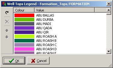
To initialise the legend, all distinct values are read from the Top Name Field
in the Well Tops table.
Double-click on an entry to edit its colour.
Delete items by clicking the  button so they will not be displayed.
Re-initialise the entire legend by clicking the  button to re-read the
formation tops table.
button to re-read the
formation tops table.
Use the  and
and  buttons to move the highlighted item in the displayed legend.
Depth Field - Select the field in the formation tops table which specifies the measured depth for your formation tops. It is assumed that the depth units are metres, and are positive values.
Top Name Field - Select the field in the formation tops table which specifies the name for each formation.
Tops Fill Style - Select the style in which the formation tops will be drawn - select from:
Solid - solid colour (defined in the well tops legend) used to fill the full depth range of each formation.
Fade to white - gradient fill starting with the well tops legend colour, and fading to white, over the depth
pixel range defined below.
Top Line - formation tops are drawn using a coloured line (colour defined in the well tops legend) at the top depth,
over a white background
Top Fade Height (px) - for 'Fade to White' above, this option defines the pixel height of the colour gradient.
Highlight Current Well on Map (checkbox) - Indicate whether to highlight the active well on the map by flashing the point.
Highlight Colour - Select a colour for the well point highlight
Highlight Width (px) - Set the radius in pixels for the current well point highlight.
Export...
Export 3D Curves - click this button to convert the LAS curves into pseudo-3D shapefiles suitable for display in ArcScene. Each well will be output to a separate shapefile, with each curve as a separate feature within the shapefile. A datum field from the well attribute table is used to ensure that measured depths have the correct vertical offset, but horizontal deviations applied to each curve polyline are purely cosmetic, to allow viewing from a single angle.
6.2 Wireline Log Viewer Window
To display wireline data, activate the Show Well Viewer tool on the
Lynx Seismap toolbar, then click a well point to launch a viewer. This tool uses ArcMap's
Selection Tolerance to select features in a similar way to ArcMap's Select Features tool,
Select By Graphics command, Edit tool and Identify tool. When you click on the map,
wells within the radius of the selection tolerance will be selected. If more than one well is selected,
a dialogue box will be displayed for you to choose which well to display.
You can also browse the attribute table of the wireline log layer to select logs to view. Open the attribute table by right-clicking on the layer in the Arcmap Table of Contents panel, then browse to the record for the log you wish to display. Right-click on the record-marker to display the Table Record Marker Context Menu, and then click View wireline curves.
Wireline Display Parameters
Wireline Display Parameters can be accessed via the Wireline Display Options
menu on the Seismap toolbar and
the Options-Display Properties menu item in wireline
viewer windows.
These parameters allow you to set display and scale parameters globally for all wireline viewer windows.
Changes made here will be applied to all currently open and subsequently open viewer windows.
- Fixed - tracks can be manually resized by dragging the gripper between each track header
- Stretch to window - all the tracks are resized dynamically to fit the current width of the viewer window - manual resizing of individual tracks is disabled.
Track Header Scrolling - change the behaviour of the track header curve scales. If there are more curves than can fit in the space allocated, the header can be scrolled using the scroll arrows above each track. Choose from hover (automatic scrolling) or click (explicit scrolling).
Curve Scalebar Baseline - YES/NO - turn on/off display of a baseline for each curve scalebar.
Initial Depth Scale - set the initial depth scale as a ratio (eg 1:10,000) used for display when a wireline log file is first opened. This scale is also used for full-scale plotting
Each well log viewer window displays the wireline curves from a single LIS/LAS file.
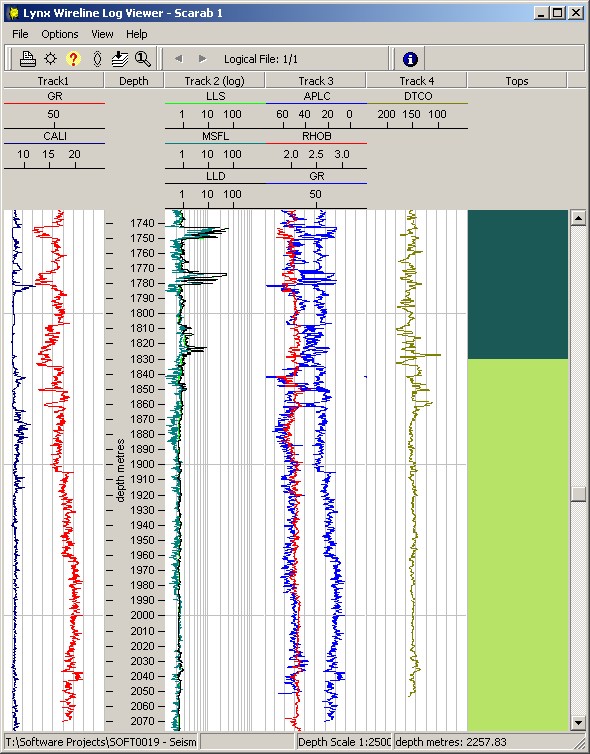
Wireline log viewer window with formation tops column
Wireline Curve Master List
The Seismap wireline log viewer shares configuration files with the standalone Lynx Logview application. You can configure a network-wide master curve list, to store layout information for all defined curves and mnemonics, plus your individual customisations are stored in a user-specific layout file in your profile folder. Changes you make to curve layouts will be visibile in both Seismap and Logview.
See the Logview help for more information about:
- Unknown Curve Mnemonics
- Track Editor and Curve Display Properties
- Defining a Master Curve List
- Synchronising changes between user layout and master curve list
6.3 Import Wireline Logs
Seismap reads wireline logs in pre-existing LAS or LIS formats. You can create a new feature class for your wireline logs in a file geodatabase or shapefile using this wizard, displayed by the Import Wireline Logs menu.
Before using this wizard, you must already have the well locations loaded as a point layer in the current ArcMap data frame. This wizard provides a simple mechanism for adding wireline log files to an ArcMap document for use with Seismap - you can also use other import and geodatabase editing facilities within ArcGIS Desktop to create Seismap wireline log layers.
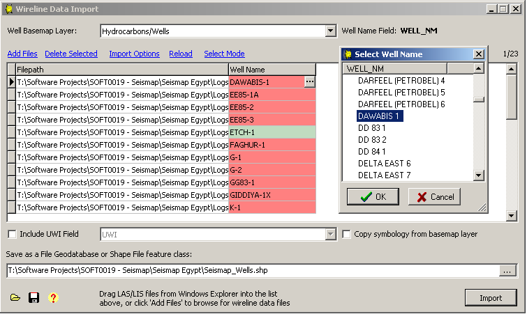
Wireline log import, showing well names highlighted red (missing), and green (OK), with wellname selection picklist
First, select your well locations layer from the drop-down list. Select from all available point layers in the current map frame.
The Import Wireline Options determine how the required information is read from the listed wireline log files.
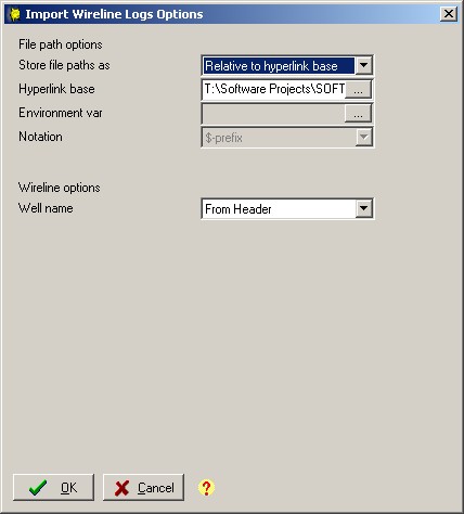
File path options
Select whether to store file paths as absolute, relative or using an environment variable.
If you choose to use relative paths, you must specify the base folder from which these relative paths
will be resolved. This will be saved as the Hyperlink Base in your MXD. If you choose to use an environment
variable, select whether to use $- or %-notation - there are advantages and disadvantages to both.
For more discussion of these options, see File name resolution (below).
Next, drag LAS/LIS files from an Explorer window onto the wizard window, or click Add Files to browse for
wireline log files. Each selected file will be added to the displayed list.
Click Delete Selected to remove selected records from the list.
Click Import Options to edit the Import 2D Seismic Options (see below).
Click Refresh to re-read filepaths and well names from the wireline log files using the current import options.
Click Edit Mode/Select Mode to switch between row-select mode, which allows you to select multiple records for deletion, and
field-edit mode, which allows you to manually edit field values in the list.
The well name for each log file will be highlighted in red or green. A red highlight means the line name is not present in the selected well basemap layer. Click the '...' button in the well name field when in Edit Mode (or press Ctrl+Enter) to display the well name picklist to select the correct well name. Well names often differ in spacing or capitalisation - you must ensure that well names match exactly for the table relationships created by Arcmap to function correctly. A green highlight means the well name is present in your selected well basemap layer.
If your existing well locations layer includes a UWI (Unique Well Identifier) attribute, you can choose to include this in your output layer in addition to the well name field. This UWI is often used to relate the well features to other tables and feature classes in your geodatabase, instead of linking on the well name. Tick the 'Include UWI Field' checkbox and select the UWI attribute field from the drop-down list.
You can also choose to copy the symbology from your selected well basemap layer to your new output wireline log layer by ticking the Copy Symbology checkbox. If the symbology depends on any of the other attribute fields, then these fields will be copied into your output feature class.
The buttons at the bottom of the wizard window allow you to save and reload the displayed list of wireline log files:
- - load an existing dBASE (DBF) file saved in this wizard.
- - save the current list as a dBASE (DBF) file.
- - display this help.
After you have added all wireline log files, and verified the well names, select a feature class destination to save this wireline log list in a File Geodatabase table or as a new shapefile.
Click Import to create your new output feature class. This will create a new feature class layer containing a copy of the point geometry (plus any additional attribute fields selected above) from your selected well basemap layer. This new layer is then added to your current ArcMap data frame. You can then activate the Select Well tool to view your wireline logs
7. Cross-Section Viewer
7.1 Cross Section Layer Properties
Raster cross-sections can be displayed for simple polyline feature classes. Seismap layer properties can be accessed as a tab in the standard Layer Properties dialog.
Use this layer for Lynx Seismap Cross Sections (checkbox) - check this box to activate Seismap for this layer and enable the rest of the parameters on this property page.
Filepath Field - select the attribute table field which contains the path of the raster file. This field must be a string field, and should contain the path to the file for each cross-section (feature). File paths are resolved in a similar way to that used for standard ArcMap hyperlinks - see File name resolution (below) for more information. Raster files can be in the following formats: TIFF (RGB, greyscale), JPEG, RLC, or PDF.
Page Number Field - for PDF documents, select then attribute table field which contains the page number of the cross-section. This field is only used for PDF cross-sections, as PDF is a multi-page format. For raster cross-sections in TIFF/JPEG/BMP format, you can ignore this parameter, or set it to <No Page Number Field>
Calibration Method - select from
- Line Ends - this calibration method assumes that the horizontal scale of the raster cross-section image is exact, and matches the length of the polyline feature. The first point of the polyline feature is assumed to correspond exactly with the top-left pixel ofthe raster image, and lengths along the cross-section are calculated as a simple ratio of total length.
- Calibration File - this calibration method is not yet implemented. It will use a triangulated calibration file to enable non-linear scales to be represented.
Cal File Field - for Calibration File method (above) - the attribute table field which contains the path to a Lynx calibration file. Not yet implemented.
Highlight Current Range on Map
(checkbox) - highlight the current viewer range on the map. The current
range is interactive - you can use the 'hand' tool
on the Lynx Seismap toolbar to grab and pan a displayed range in ArcMap's data view.
Highlight Colour - Select a colour for the current cross-section range highlight
Highlight Width (px) - Set the width in pixels for the current range highlight.
7.2 Cross-Section Raster Viewer Window
To display raster and PDF cross-sections, activate the Show Cross-Section
tool on the Seismap toolbar,
then click a cross-section feature in the map view to view the associated cross-section. This tool uses
ArcMap's Selection Tolerance to select features in a similar way to ArcMap's Select Features tool,
Select By Graphics command, Edit tool and Identify tool. When you click on the map, polyline features
within the radius of the selection tolerance will be selected. If more than one feature is selected, a dialogue
box will be displayed for you to choose which cross-section to display. Note that the feature's primary
display field must be set, and must contain a non-null value, as this is used as the cross-section viewer title.
Multiple windows can be open viewing different profiles at the same time.
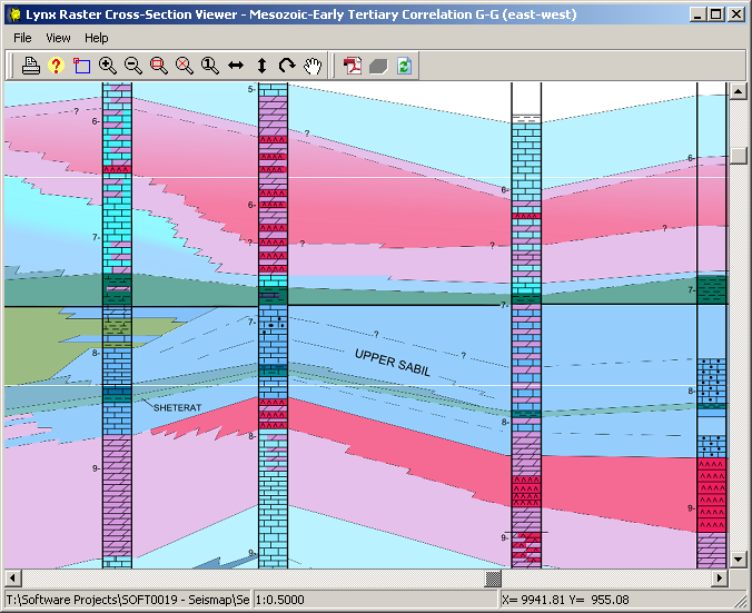
The displayed range of the cross-section will be highlighted on the map, and you can use the Seismap Pan tool to move the displayed range. You can also use the zoom and pan tools on the cross-section viewer toolbar manipulate the current view.
When the current cross-section is a page from a PDF file, the PDF Toolbar is activated (these options are also available in the View menu):
 Display PDF Document - open the whole PDF document in your default PDF viewer
application. The icon displayed in this toolbar may vary depending on your default PDF viewer application.
Display PDF Document - open the whole PDF document in your default PDF viewer
application. The icon displayed in this toolbar may vary depending on your default PDF viewer application. Show/Hide PDF Layers - if the PDF document contains layered content, you
can turn individual layers on/off.
Show/Hide PDF Layers - if the PDF document contains layered content, you
can turn individual layers on/off. Reload PDF - re-read the page from the PDF document file.
7.3 Import Cross-Sections
You can associate cross-sections in raster format or as individual pages in PDF files, with lines of cross-section which already exist as polyline layer. The Import Cross-Sections wizard provides a simple mechanism for adding cross-sections to an ArcMap document for use with Seismap - you can also use other import and geodatabase editing facilities within ArcGIS Desktop to create Seismap cross-section layers.
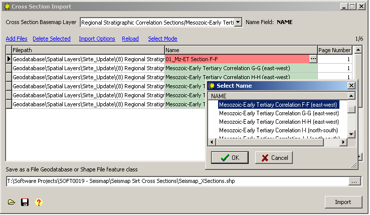
Cross-section import, showing cross-section names highlighted red (missing), and green (OK), with selection picklist
First, select your cross-section basemap layer from the drop-down list. Select from all available polyline layers in the current map frame.
The Import Cross-Section Options determine how the required information is read from the listed raster files.
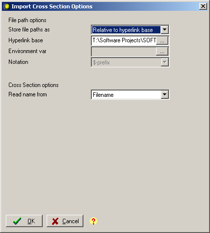
File path options
Select whether to store the file paths as absolute, relative or using an environment variable.
If you choose to use relative paths, you must specify the base folder from which these relative paths
will be resolved. This will be saved as the Hyperlink Base in your MXD. If you choose to use an environment
variable, select whether to use $- or %-notation - there are advantages and disadvantages to both.
For more discussion of these options, see File name resolution (below).
Next, drag raster or PDF files from an Explorer window onto the wizard window, or click Add Files to browse for
files to add. Each selected file will be added to the displayed list.
Click Delete Selected to remove selected records from the list.
Click Import Options to edit the Import 2D Seismic Options (see below).
Click Refresh to re-read filepaths and well names from the wireline log files using the current import options.
Click Edit Mode/Select Mode to switch between row-select mode, which allows you to select multiple records for deletion, and
field-edit mode, which allows you to manually edit field values in the list.
The cross-section name for each file will be highlighted in red or green. A red highlight means the name is not present in the selected cross-sections basemap layer. Click the '...' button in the Name field when in Edit Mode (or press Ctrl+Enter) to display the Name picklist to select the correct Name. You must ensure that well names match exactly for the import process to function correctly. A green highlight means the Name is present in your selected cross-sections basemap layer.
For PDF files, you can also edit the Page Number field for each added file. This is the page that contains the cross-section image to be displayed. Page numbers in PDF files are always counted from the first page in the document 1. The page number field is not used for raster formats (TIFF, JPEG, BMP).
The buttons at the bottom of the wizard window allow you to save and reload the displayed list of cross-sections:
- - load an existing dBASE (DBF) file saved in this wizard.
- - save the current list as a dBASE (DBF) file.
- - display this help.
After you have added all cross-section files, and verified the names and page numbers, select a feature class destination to save this cross-section list in a File Geodatabase or as a new shapefile.
Click Import to create your new output feature class. This will create a new feature class layer containing a copy of the polyline geometry from your selected cross-section basemap layer. This new layer is then added to your current ArcMap data frame. You can then activate the Select Cross-Section tool to view your sections
8. Filename Resolution
The files used by all Seismap layers must be referenced in the layer's attribute table. There are three ways in which you can define file paths:
File paths on Windows are not usually case sensitive.
8.1 Absolute paths
Absolute paths start with either a drive-letter or a UNC share-name:
eg
M:\GIS\Libya\Seismic\SEGY\10BR-70.STK
\\server_1\vol1\GIS\Libya\Seismic\SEGY\10BR-70.STK
Absolute filepaths are usually unique to your network environment or your local PC. If you move the MXD or geodatabase to a different folder path or network drive, the your referenced absolute filepaths will not have to be relocated. Absolute filepaths work best when you have multiple MXDs in different network locations pointing to a single reference dataset.
8.2 Relative paths
Relative paths do not start with a drive-letter or UNC share-name. These are resolved using the hyperlink base for the MXD if this is set, otherwise they will be resolved from the folder containing the current MXD file.
Relative paths enable the whole GIS 'package' to be moved to a different network location or folder as a single unit. You can create multiple working copies of the dataset.
8.3 Environment variables
Environment variables are dynamic named values which can be set for individual users and individual PCs. Define a new environment variable to allow customising of the path to your data files. Different users or different network environments may require a different network filepath to be used to access the same data, or the GIS 'package' may be located in different folder locations on the C: drive for different users.
Environment variables are one method of resolving different drive mappings between different PCs on a network, or accessing data on removable drives (CD-ROM, DVD and USB devices) which may use a different drive letter on different PCs. Seismap supports two notations for including environment variables in paths - you can include an environment variable in your path specification using either $ or % notation.
$-notation is the historical standard for UNIX, and is compatible with the rest of ArcMap and ArcView 3. If you need to use standard ArcMap hyperlinks as well as Seismap, then you will need to use this format. A path including an environment variable using $-notation would look something like $LIBDATA\Seismic\SEGY\10BR.STK where the environment variable LIBDATA is set to M:\GIS\Libya.
%-notation is the Windows standard, but is not recognised by standard ArcMap hyperlinks. A path including an environment variable using %-notation would look something like %LIBDATA%\Seismic\SEGY\10BR.STK.
Lynx provides the SetEnvVar tool to simplify the creation and editing of user-specific environment variables from within ArcMap, without the need to restart.
Alternatively, to set an environment variable you can use the standard Windows dialog: in XP right-click on My Computer on the desktop or in Explorer and select Properties; in Windows 7 open the start menu and type sysdm.cpl in the search box. Select the Advanced tab and click the Environment Variables button.
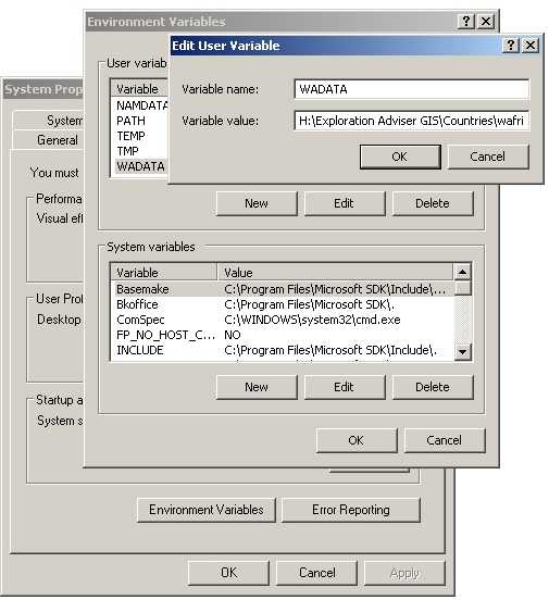
To set the environment variable for just the current logged-on
user, click the New button underneath the User variables
list. To set the environment variable for all users who log on to this
PC, click the New button underneath the System variables list
(you will need administrative privileges for this). Enter the environment
variable name, and the file path to substitute for it. Do not include $ or %
characters in the variable name in this dialogue.
Alternatively, you can set environment variables by using a login script.
After setting or changing environment variables, you will need to restart ArcMap for any
changes to be recognised.
See also:
- UKO2SHP - UKOOA to Feature Class Converter
- SEISVIEW - Lynx Seismic Viewer
- Seismic 3D Inline Display
- LOGVIEW - Lynx Wireline Log Viewer
- Viewer Common Functionality
- LEA Software Licensing
- PRMEDIT - Lynx Parameter Editor
- FILEREG - Lynx File Registration Utility
- Main Index
Copyright © Lynx Information Systems Ltd 2020